Silhouette width partial computation
Table of Contents
Summary
- Summary
- Introduction
- Definition of the silhouette width
- Calculating the silhouette width
- Comparison
- Full code
Introduction
The silhouette width is an internal cluster validity index that was first proposed in Rousseeuw (1987)1. It uses the average intra-cluster distances and inter-cluster separation to indicate whether a data point (or object) is likely to be in the right cluster. This has the utility of providing a number in the range $[-1,1]$, where a positive value indicates that a point is likely to have been assigned to the right cluster (as it is on average closer to the other points in its cluster than to any other cluster).
One issue with the silhouette width is its complexity - $O(DN^{2})$, where $D$ is the dimensionality and $N$ is the number of data points. One useful property we can exploit to reduce the computation needed is that the majority of the pairwise distances (which are used in the silhouette width) are unlikely to change following a small perturbation to the data.
An application for the partial computation is in my synthetic cluster generator, HAWKS, where it is used as the fitness function. As the core of HAWKS is a genetic algorithm, we have a population of individuals (datasets), and so the silhouette width needs to be calculated for each individual in the population every generation. Needless to say, this has the potential to make the evolution very slow. Fortunately, changes in the individuals are caused by crossover and mutation only. Neither of these operators are guaranteed to occur, and they operate on a subset of the clusters, thus changing only a subset of the pairwise distances.
Another potential application is when using the silhouette width for data stream clustering, an area of research of increasing prevalence. For some situations, there may be minor changes to the dataset, either through the modification of a subset of the data, or through the introduction of a small (relative to the overall size) number of data points.
This post will explain the silhouette width, how it is typically calculated, and how we can utilize this partial computation to reduce computation.
Definition of the silhouette width
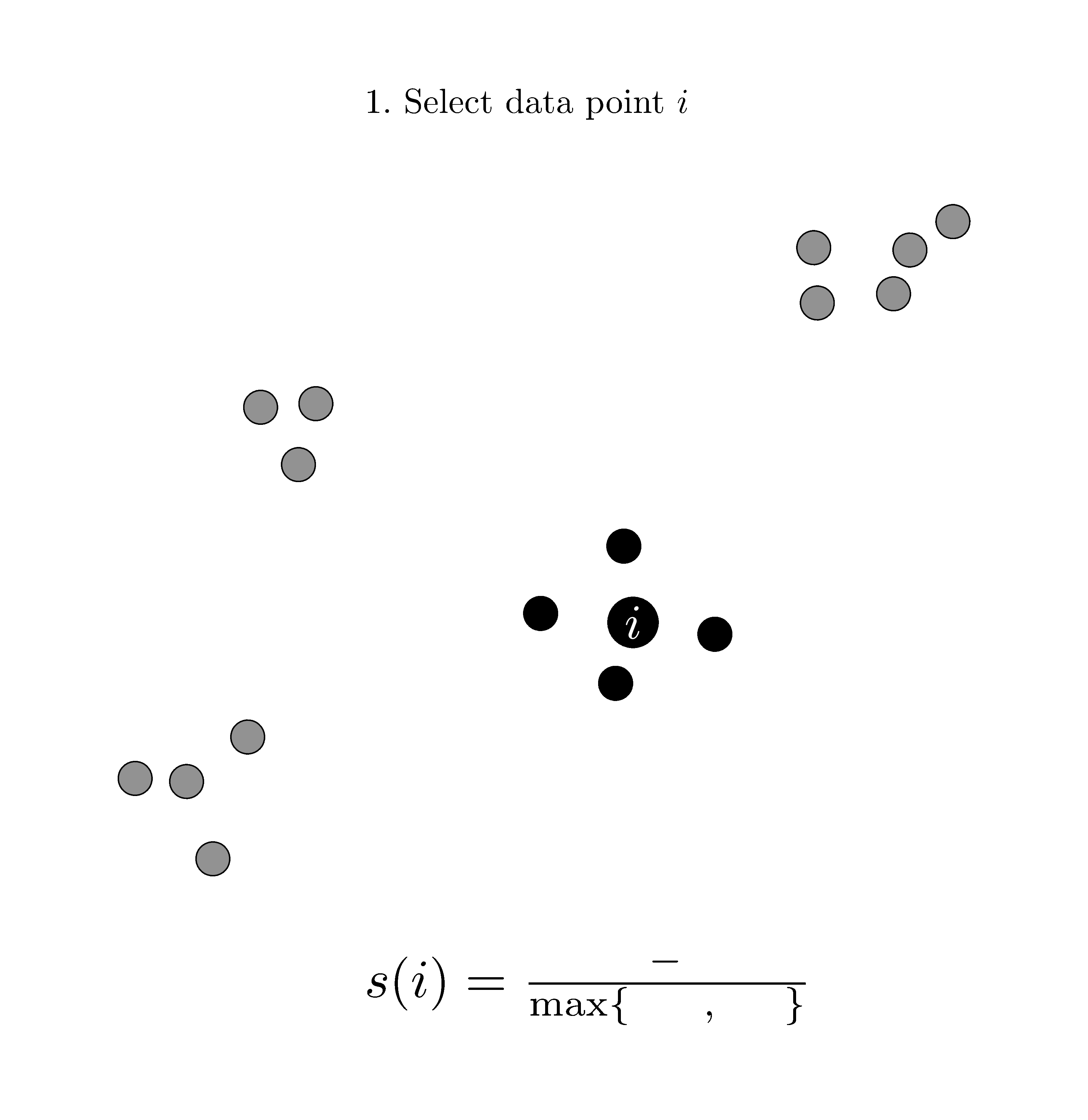
The silhouette width is calculated for a single data point (or object), $i$, and is defined as follows:
$$ s(i) = \frac{{b(i)} - a(i)}{\max\{a(i),b(i)\}} $$
where $a(i)$ represents the cluster compactness (with respect to object $i$) and $b(i)$ represents minimum average separation from $i$ to another cluster. The standardisation achieved by the denominator term keeps $s(i)$ in the range $[-1,1]$. For $a(i)$, we calculate the average distance from $i$ to all other objects in its cluster:
$$ a(i) = \frac{\sum_{j\in C_{k}}~d{(i,j)}}{| C_{k} | - 1} \qquad ~i\neq j;~i \in C_{k};~C_{k} \in \mathcal{C} $$
where $\left | C_{k} \right |$ is the $k$th cluster’s cardinality, $\mathcal{C} = \{C_{1},\ldots,C_{K}\}$ is the set of $K$ clusters, and $d{(i,j)}$ is the distance (typically Euclidean) between objects $i$ and $j$. We divide by $| C_{k} | - 1$ as $d(i,i)$ is not included.
We then calculate $b(i)$ as:
$$ b(i) = \min_{\forall C_{k} \in \mathcal{C}} \frac{\sum_{j\in C_{k}}~d{(i,j)}}{\left | C_{k} \right |} \qquad ~i \notin C_{k}. $$
Note that the silhouette width for a singleton cluster (i.e. $|C_{k}|=1$ and $i \in C_{k}$) is defined as $s(i) = 0$.
The different parts of this equation and how they relate can be seen in the following GIF:
To get the average silhouette width for the dataset, $s_{\text{all}},$2 we then take the average $s(i)$ across all $N$ data points:
$$ s_{\text{all}} = \frac{1}{N} \sum_{i=1}^{N} s(i). $$
Calculating the silhouette width
In this section I’ll go over the full and then a reduced computation version of the silhouette width. You can skip to the full code, or see it implemented in HAWKS here.
Full calculation
I’ll show how we can compute this in numpy/scipy, though there is an implementation available in sklearn here. Note that I’ve tried to make the implementation shorter by just making every cluster the same size.3
Let’s assume we have a small dataset of $N=9$ and $K=3$, where each cluster contains three objects. The distance matrix (pairwise distances between all points) is a $N \times N$ symmetric matrix, with 0 on the diagonal (as the distance between a point and itself is 0). The blocks below show which part of the distance matrix corresponds to the different parts of the silhouette width calculation. For our purposes, the objects that belong in the same cluster are contiguous in the distance matrix, though thanks to numpy this isn’t a requirement.

Calculating the pairwise distances is simple enough, thanks to scipy. One thing to note is that scipy uses a vector-form distance vector, rather than a full distance matrix, which would be more appropriate as $N$ grows. Using squareform with pdist slows things down, but it can be more intuitive to work with full distance matrices, so we’ll do that here. For details, see here.
# Initial imports
from itertools import permutations
from collections import defaultdict
import numpy as np
from scipy.spatial.distance import pdist, squareform

def full_distances(data, metric="sqeuclidean"):
    return squareform(pdist(data, metric=metric))
For efficiency, we calculate $s(i)$ for every $i$ simultaneously. We start with $a(i)$, or the intra-cluster distances. Here, we select each of the relevant blocks on the diagonal of the distance matrix (as previously shown), then divide the sum of these distances by the cardinality (i.e. size) of the cluster.
def full_intraclusts(dists, N, cluster_size):
    # Calculate the intracluster variance
    a_vals = np.zeros((N,))
    # Loop over each cluster (exploit equal size)
    for start in range(0, N, cluster_size):
        # Get the final index for that cluster
        stop = start+cluster_size
        # Get the relevant part of the dist array
        clust_array = dists[start:stop, start:stop]
        # Divide by the cardinality
        a_vals[start:stop] = np.true_divide(
            np.sum(clust_array, axis=0),
            stop-start-1 # As we don't include d(i,i)
        )
    return a_vals
Calculating the minimum inter-cluster distances, $b(i)$, is slightly trickier. We need to calculate, for each data point, the average distance to every point in every other cluster, and then select the minimum of these averages. To get all the 2-tuple permutations of the clusters, we use itertools.permutations. We initialize the $b(i)$ values vector to np.inf so that if anything is unfilled, we’ll get a warning later on. We could just use a single vector (of length $N$) for b_vals, keeping the minimum as we iterate over each cluster. Here, however, we are using a $N \times K$ matrix instead, as this is more useful later on in the partial calculation.
For each cluster, we calculate the relevant indices to get the appropriate submatrix of the distance matrix. Then, we just calculate the mean distances to that cluster and store it in the column for that cluster. We can then later select the minimum from the $K$ columns.
def full_interclusts(dists, N, K, cluster_size):
    # Calculate the intercluster variance
    # Get the permutations of cluster numbers
    perms = permutations(range(K), 2)
    # Initialize the b_values
    # Default to np.inf so we get a warning if it doesn't work
    b_vals = np.full((N, K), np.inf)
    # Calc each intercluster dist
    for c1, c2 in perms:
        # Get indices for distance array
        c1_start = c1*cluster_size
        c1_stop = c1_start+cluster_size
        c2_start = c2*cluster_size
        c2_stop = c2_start+cluster_size
        # Get the relevant part of the dist array
        clust_array = dists[c1_start:c1_stop, c2_start:c2_stop]
        # Select the minimum average distance
        b_vals[c1_start:c1_stop, c2] = np.mean(clust_array, axis=1)
    return b_vals
Putting it all together, we can calculate the silhouette width as follows:
def full_silh(data, N, cluster_size, K):
    # Get the distances
    dists = full_distances(data)
    # Calculate the main terms
    a_vals = full_intraclusts(dists, N, cluster_size)
    b_vals = full_interclusts(dists, N, K, cluster_size)
    # Select the minimum average distance
    b_vec = b_vals.min(1)
    # Calculate the numerator and denominator
    top_term = b_vec - a_vals
    bottom_term = np.maximum(b_vec, a_vals)
    res = top_term / bottom_term
    # Handle singleton clusters
    res = np.nan_to_num(res)
    return np.mean(res), dists, a_vals, b_vals
Let’s validate that our method of calculating works:
def test_full():
    # Set random seed
    np.random.seed(42)
    # Setup variables
    N, D, K = 1000, 2, 10
    cluster_size = int(N/K)
    data, labels = random_data(cluster_size, D, K)
    # Calculate the silhouette widths
    our_sw = full_silh(data, N, cluster_size, K)
    sk_sw = silhouette_score(data, labels, metric='sqeuclidean')
    print(f"Our method:   {our_sw}")
    print(f"Scikit-learn: {sk_sw}")
    assert np.isclose(our_sw, sk_sw)
Our method:   0.8039652717646208
Scikit-learn: 0.8039652717646208
Fortunately, we get the same as sklearn, so assuming we don’t both have the exact same bug we can move on.
Partial calculation
Now we can look at refining this so that we only recompute what is needed, following a partial change in the data. When a single cluster changes, the pairwise distances in corresponding rows/columns for those data points in the distance matrix also change. Therefore, only the $a(i)$ values in the clusters that change need to be recomputed, and the cluster combinations in $b(i)$ which include a modified cluster (this is where storing all $K$ values for each data point in b_vals pays off).
In our scenario, the cluster change results from a perturbation (from crossover or mutation), and so we know which clusters have changed. Therefore, we know which subsets of the distance matrix need recomputation, which we can do as follows:
def partial_distances(data, dists, cluster_size, changed_clusters, metric="sqeuclidean"):
    for i, changed in enumerate(changed_clusters):
        # Skip if unchanged
        if not changed:
            continue
        # Get the indices for the cluster
        start = i*cluster_size
        stop = start+cluster_size
        # Calculate the new block of pairwise matrices
        new_dists = cdist(
            data,
            data[start:stop, :],
            metric=metric
        )
        # Insert the new distances (in both as symmetric)
        dists[:, start:stop] = new_dists
        dists[start:stop, :] = new_dists.T
    return dists
The actual functions for the calculation $a(i)$ is mostly identical, but the list of clusters that have changed is used to skip the clusters that don’t require recalculation:
def partial_intraclusts(a_vals, dists, N, cluster_size, changed_list):
    # Loop over each cluster (exploit equal size)
    for clust_num, changed in enumerate(changed_list):
        if not changed:
            continue
        # Get the indices for the cluster
        start = cluster_size * clust_num
        stop = start + cluster_size
        # Get the relevant part of the dist array
        clust_array = dists[start:stop, start:stop]
        # Divide by the cardinality
        a_vals[start:stop] = np.true_divide(
            np.sum(clust_array, axis=0),
            stop-start-1 # As we don't include d(i,i)
        )
    return a_vals
For the $b(i)$ values, a change in any single cluster requires some recalculation for every other cluster, but only a subset of the possible combinations need to be done. For example, in the annotated distance matrix below we can see that if $C_{3}$ were changed, anything that involves $C_{3}$ needs recalculation to see if there is a new minimum.

So, for each cluster that has changed, we can loop over every other cluster and then update the relevant parts of the b_vals matrix as shown below:
def partial_interclusts(b_vals, dists, K, cluster_size, changed_list):
    # Loop over the clusters that have changed
    for c1, changed in enumerate(changed_list):
        if changed:
            # Determine the relevant indices
            c1_start = c1 * cluster_size
            c1_stop = c1_start + cluster_size
            # Loop over every other cluster
            for c2 in range(K):
                if c1 == c2:
                    continue
                # Get indices for distance array
                c2_start = c2 * cluster_size
                c2_stop = c2_start + cluster_size
                # Get the relevant part of the dist array
                clust_array = dists[c1_start:c1_stop, c2_start:c2_stop]
                # Set the minimum average distance for the c1,c2 combo
                b_vals[c1_start:c1_stop, c2] = np.mean(clust_array, axis=1)
                # Set the minimum average distance for the c2,c1 combo
                b_vals[c2_start:c2_stop, c1] = np.mean(clust_array, axis=0)
    return b_vals
Putting it all together, our overall function can enable both full and partial recomputation:
def partial_silh(data, N, cluster_size, K, changed_list=None, dists=None, a_vals=None, b_vals=None):
    if changed_list is None:
        changed_list = [True]*K
    # Get the distances
    if dists is None:
        dists = full_distances(data)
    else:
        dists = partial_distances(data, dists, cluster_size, changed_list)
    # Allows us to use this function for the first calc
    if a_vals is None:
        a_vals = np.zeros((N,))
    if b_vals is None:
        b_vals = np.full((N, K), np.inf)
    # Calculate the main terms
    a_vals = partial_intraclusts(a_vals, dists, N, cluster_size, changed_list)
    b_vals = partial_interclusts(b_vals, dists, K, cluster_size, changed_list)
    # Select the minimum average distance
    b_vec = b_vals.min(1)
    # Calculate the numerator and denominator
    top_term = b_vec - a_vals
    bottom_term = np.maximum(b_vec, a_vals)
    res = top_term / bottom_term
    # Handle singleton clusters
    res = np.nan_to_num(res)
    return np.mean(res), dists, a_vals, b_vals
Now let’s check that our new functions work by first calculating the full silhouette width, and then modifying two clusters and running it again using the partial computation.
def test_partial():
    # Set random seed
    np.random.seed(42)
    # Setup variables
    N, D, K = 1000, 2, 10
    cluster_size = int(N/K)
    data, labels = random_data(cluster_size, D, K)
    changed_list = [True]*K
    # Need to first do the full calculation
    our_sw, dists, a_vals, b_vals = partial_silh(data, N, cluster_size, K, changed_list)
    # Compare with the full scikit calc to check
    sk_sw = silhouette_score(data, labels, metric='sqeuclidean')
    assert np.isclose(our_sw, sk_sw)
    # Drastically change the first cluster
    data[:100] = np.random.multivariate_normal(
        mean=[np.random.rand() * 1000 for _ in range(D)],
        cov=np.eye(D),
        size=cluster_size
    )
    # Drastically change the third cluster
    data[200:300] = np.random.multivariate_normal(
        mean=[np.random.rand() * 500 for _ in range(D)],
        cov=np.eye(D),
        size=cluster_size
    )
    # We changed the first and third cluster
    changed_list = [True, False, True, False, False]
    # Now partially recalculate the silhouette width
    our_sw, _, _, _ = partial_silh(data, N, cluster_size, K, changed_list, dists, a_vals, b_vals)
    sk_sw = silhouette_score(data, labels, metric='sqeuclidean')
    print(f"Partial method: {our_sw}")
    print(f"Full method:    {full_silh(data, N, cluster_size, K)[0]}")
    print(f"Scikit-learn:   {sk_sw}")
    assert np.isclose(our_sw, sk_sw)
Partial method: 0.8991699790956502
Full method:    0.8991699790956502
Scikit-learn:   0.8991699790956502
Great! Now, we can look at whether all of this was actually worth it (in terms of computation, at least).
Comparison
To see if the partial calculation is worth it, we need to compare the run times between the full method, the partial method, and the sklearn method when run first on the dataset, and then again after the data has been modified. By varying some different parameters, such as the proportion of clusters that are being changed, the size of the dataset ($N$) and the dimensionality ($D$), we will see if there is a point where the overhead of partial computation outweighs the savings. After all, matrix multiplications are awfully efficient, and the overhead we have created with for loops is, well, potentially less efficient. If the proportion of clusters that change is large, it could quite reasonably be that restarting and calculating the full silhouette width is more efficient.
To ensure a robust timing, each method is run 10 times, and the average time is taken. Here is the code for the experiment:
def random_data(cluster_size, D, K):
    data_list = []
    for k in range(K):
        # Generate some random normal data
        data = np.random.multivariate_normal(
            mean=[np.random.rand() * 5 * k for _ in range(D)],
            cov=np.eye(D),
            size=cluster_size
        )
        # Append labels to the data
        # Note that this is only needed for the partial computation
        data = np.hstack((data, np.full((cluster_size, 1), k)))
        # Add the data to our list
        data_list.append(data)
    # Create a single array of the data
    full_data = np.concatenate(data_list)
    labels = full_data[:, -1]
    return full_data[:, :-1], labels

def modify_data(data, changed_list, cluster_size, D):
    new_data = data.copy()
    for i, changed in enumerate(changed_list):
        if changed:
            start = i*cluster_size
            stop = start + cluster_size
            new_data[start:stop] = np.random.multivariate_normal(
                mean=[np.random.rand() * np.random.randint(100, 1000) for _ in range(D)],
                cov=np.eye(D),
                size=cluster_size
            )
    return new_data

def add_result(res, N, D, K, changes, method, time):
    res["# Examples"].append(N)
    res["Dimensionality"].append(D)
    res["Number of Clusters"].append(K)
    res["Proportion Changes"].append(changes)
    res["Method"].append(method)
    res["Time (s)"].append(time)
    return res

def time_comparison(Ns, Ds, Ks, changes_list):
    params = product(Ns, Ds, Ks, changes_list)
    res = defaultdict(list)
    repeats = 10
    # Loop over param combs
    for N, D, K, changes in params:
        cluster_size = int(N/K)
        data, labels = random_data(cluster_size, D, K)
        # Simulate expected mutations
        changed_list = [True if np.random.rand() < (changes/K) else False for _ in range(K)]
        # Just modify it the once so it doesn't interfere with timing
        new_data = modify_data(data, changed_list, cluster_size, D)

        for _ in range(repeats):
            # Full calculation
            start = time.time()
            # Run initial
            test = full_silh(data, N, cluster_size, K)
            # Run on mutated data
            full_sw, _, _, _ = full_silh(new_data, N, cluster_size, K)
            full_time = time.time() - start
            # Store the result
            res = add_result(res, N, D, K, changes, "Full", full_time)

            # Partial calculation
            start = time.time()
            # Run initial
            test2, dists, a_vals, b_vals = partial_silh(data, N, cluster_size, K)
            # Run on mutated data
            partial_sw, _, _, _ = partial_silh(new_data, N, cluster_size, K, changed_list, dists, a_vals, b_vals)
            partial_time = time.time() - start
            # Store the result
            res = add_result(res, N, D, K, changes, "Partial", partial_time)

            # sklearn calculation
            start = time.time()
            _ = silhouette_score(data, labels, metric='sqeuclidean')
            sklearn_sw = silhouette_score(new_data, labels, metric='sqeuclidean')
            sk_time = time.time() - start
            # Store the result
            res = add_result(res, N, D, K, changes, "sklearn", sk_time)

            # Check that all the results are the same
            assert np.isclose(full_sw, partial_sw) and np.isclose(partial_sw, sklearn_sw)

    df = pd.DataFrame(res)
    df.to_csv("sw_times.csv")
    return df

def plot_times(df):
    # Construct a facetgrid
    g = sns.FacetGrid(
        data=df.groupby(["# Examples", "Dimensionality", "Proportion Changes", "Method"])["Time"].mean().reset_index(),
        row="# Examples",
        col="Dimensionality",
        hue="Method",
        margin_titles=True
    )
    # Plot the data
    g = g.map(plt.plot, "Proportion Changes", "Time", marker=".").set(yscale="log")
    g = g.add_legend()
    # Save the results
    g.savefig("sw_times.png", dpi=600)
Results
Below is the plot of results across our different parameters:
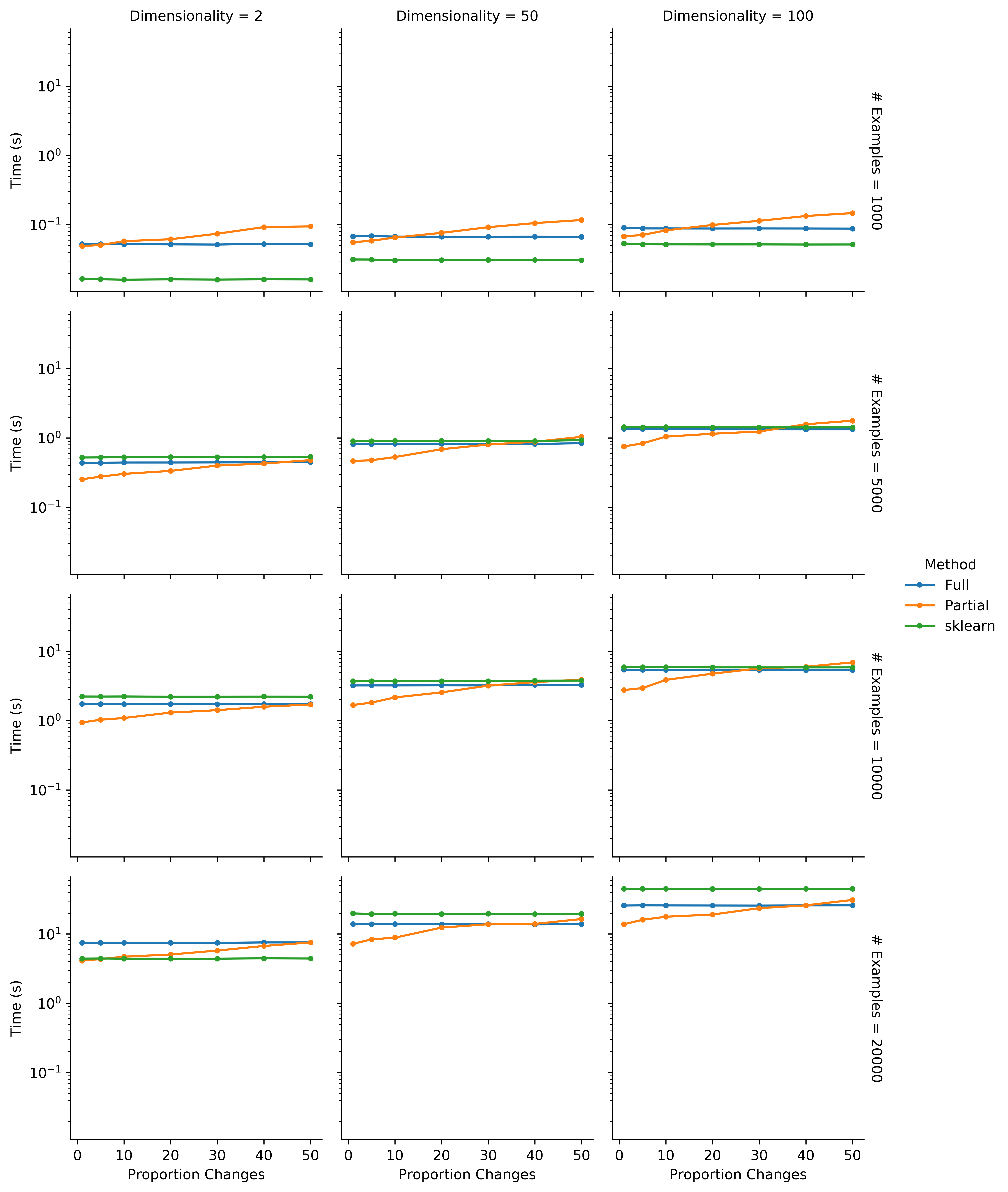
As expected, the partial computation does reduce the time, but with diminishing and even adverse effects as we increase the proportion of clusters that are being changed. Fortunately in HAWKS, each individual has on average a single change, so we’re on the far left-hand side of the x-axis. Our partial method is about twice the speed of the full computation, becoming increasingly useful as $D$ and $N$ increase. Not groundbreaking, but practically useful.
Interestingly, it seems that sklearn is faster for smaller datasets (both in terms of $N$ and $D$), but our full computation is faster as either increases. Although beyond the scope of this post, I would be interested to see if the sklearn approach is more memory efficient (I believe it is), and when used properly on a server its use of chunking/joblib can help a lot to explicitly distribute compute.
Full code
The full code is available as a GitHub gist. It is mostly for illustration, however. The code in HAWKS is a little neater, but I would also recommend checking out scikit-learn’s source code for another way of doing it, where they also have some great extras that can save on memory (and use joblib to explicitly parallelize chunks of the distance matrix).
Rousseeuw, Peter J. “Silhouettes: a graphical aid to the interpretation and validation of cluster analysis.” Journal of computational and applied mathematics 20 (1987): 53-65. ↩︎
I use $s_{\textit{all}}$ for this, though I have seen $\tilde{s}$ used. ↩︎
This is quite unrealistic, but relatively simple to change. In HAWKS, we just maintain a list of tuples, denoting the start and end indices for each cluster. We could just create this at the start, and pass this object to our function and use that instead, but to minimize code and variables I’m making the cluster sizes equal. ↩︎
Cameron Shand
Research Fellow in Disease Progression Modelling and Machine Learning for Clinical Trials
My research interests include (primarily unsupervised) machine learning, evolutionary computation, the utility of complex synthetic data, and how this can be used to further medicine.